Hilbert Neural Operators (HNO)

Introduction to Hilbert Neural Operator, a new approach regarding Neural Operators, Deep Learning architectures, tailored for scientific modelling and computational physics.

• 📄 Arxiv Preprin
• 💻 GitHub Repository

Following the new trend of deep learning specification for solving scientific problems such as simulation, forecasting, and control, which resulted to some technologies for this field like Physics-Infomed-Neural-Networs (PINN) [1], DeepONet [2], and Neural Operators [3], we are trying to test and present one of our ideas in this field following to the neural operators, which is Hilbert Neural Operator. The development of HNO is primarily motivated by the hypothesis that the Hilbert transform possesses unique properties, such as its ability to provide instantaneous amplitude and phase information through the analytic signal. This relationship might offer specific advantages for learning certain classes of operators that are not fundamentally captured by Fourier methods [4].

Neural Operators

Teaching Networks to Recognize Functions 💡

A neural operator’s typical job is mapping between fixed-size vectors, such as F: R → R. This is common when your data is a function defined on a continuous domain, like an initial condition for a PDE. The issue arises when you change the discretization grid; the network often fails.

In short, neural operators address this by directly mapping between the function space, G: A → U. Neural operators are discretization-invariant, meaning the mesh isn’t a hard-coded parameter in your network. You can train on resolution A and then test on a different resolution B.

The Core Architecture

A neural operator G approximates the true, complex operator G by stacking layers that update a function representation.

This process includes:

1. Lifting: A local network P which lifts the input function a(x) to a higher-dimensional latent space:

$$v_0(x) = P(a(x))$$

1. Kernel Integration: The core of the neural operator is an iterative spectral convolution. Each layer updates the function v(x) by applying a non-local integral operator and a local non-linearity sigma:

   $$v_{t+1}(x) = \sigma \left( W v_t(x) + \int_{\mathcal{D}} \kappa_\theta(x, y) v_t(y) \, dy \right)$$

   The kernel K enables the model to aggregate information about the incoming signal across the entire domain D, capturing more global features of the signal than local ones. Different architectures of neural operators, such as the Fourier Neural Operator (FNO) [4] and what we propose here as HNO, are defined by how they efficiently parameterize this kernel.

2. Projection: A final local network Q projects the latent function u(x) back to the desired output function:

$$u(x) = Q(v_T(x))$$

This approach and point of view on the learning problem are capable of learning the underlying continuous physics or mathematical structures, and provide a powerful, yet flexible, tool for Scientific Machine Learning.

Let’s build up some mathematical fundamentals about the Hilbert Transform:

Hilbert Transform

The Hilbert transform is defined as a specific singular integral operation that takes a function of a real variable and produces another function of a real variable. Mathematically, the Hilbert transform of a function u(t), denoted by H(u)(t) or û(t), is defined as the Cauchy principal value of the convolution of u(t) with the function:

$$h(t) = \frac{1}{\pi |t|}$$

This can be expressed as:

$$\hat{u}(t) = H(u)(t) = \frac{1}{\pi} \, \text{p.v.} \int_{-\infty}^{\infty} \frac{u(\tau)}{t - \tau} \, d\tau$$

in frequency domain:

$$\sigma_H(\omega) = -i \cdot \operatorname{sgn}(\omega)$$ $$\hat{U}(\omega) = -i \, \operatorname{sgn}(\omega) \, U(\omega)$$

complex-valued signal

$$s_A(t) = s(t) + j \hat{s}(t)$$

A fundamental property of the Hilbert transform is its effect on the phase of a signal. As mentioned earlier, it imparts a ±90 (±π/2 radians) phase shift to each frequency component.This phase-shifting property is key to many applications of the Hilbert transform in signal processing and communications.

The Hilbert transform operates both as a convolution in the time domain and as a phase shifter in the frequency domain, making it valuable for neural operator frameworks. The non-causal nature (with impulse response h(t)=1/(πt)) requires practical approximations for real-time systems. HNO’s connection to analytic signals makes it particularly useful for problems involving instantaneous amplitude and phase analysis.

Impact of the Hilbert Transform on Signals in Signal Processing

Instantaneous amplitude (or envelope) and instantaneous phase attributes are particularly useful for analyzing signals whose characteristics change over time, making HNO a potentially valuable tool for analyzing non-stationary signals.

A key property between a signal and its Hilbert transform is their orthogonality. For a signal x(t) and its Hilbert transform x^(t), the integral of their product over all time is zero.

$$\int_{-\infty}^{\infty} x(t) \hat{x}(t) \, dt = 0$$

The orthogonality results from the Hilbert transform’s 90-degree phase shift property. When forming an analytic signal, the transform removes negative frequency components, leading to more efficient signal processing.

Convolution in Hilbert Space

Now, we can get to the core of our method, which is a Hilbert-based convolution kernel. The purpose is to learn a non-linear mapping from an input function space to an output function space. To achieve this, the kernel first transforms the input into its analytic signal using the Hilbert transform. A learnable convolution will be executed in this new domain, allowing the model to operate directly on the signal’s instantaneous amplitude and phase features.

$$H^{-1}\big(H(K * v(t))\big) = H^{-1}\big(K(t) * H(v(t))\big)$$

After the convolution in the Hilbert space, we bring back the signal into its original space via the inverse Hilbert transform.

Although the main transform here is Hilbert, we’ve decided to execute the convolution operation in the Fourier space and use the advantage of the Fourier convolutional features, which convert a heavy convolution operation into a simple dot product. This approach enables us to leverage some Fourier space features, such as selecting the most significant modes, by specifying an appropriate number of modes as an additional argument.

The final spectral convolution formulation should be:

$$H^{-1} \left( F^{-1} \left( F(K * H(v(t))) \right) \right)$$

Resulted in:

$$H^{-1} \left( F^{-1} \left( F[K] \cdot F[H(v(t))] \right) \right)$$

The general overview of the network looks like the following:

The network first lifts the input signal a(x) to a high-dimensional latent space using a linear projection, P. The argument T Represents the number of HNO layers. Within each layer, the signal is processed by two parallel branches: (1) a local branch, which uses a standard convolution to capture short-range dependencies, and (2) a global branch, which employs our Hilbert spectral convolution. This global path is designed to learn the operator by extracting features based on the signal’s instantaneous phase and amplitude, for capturing long-range interactions. The outputs of these two branches are then combined via summation, followed by a non-linear activation function. After the final HNO layer, a projection layer, Q, maps the latent representation back to the desired output dimension, retrieving the final output u(x).

Experiment and Results

Our full experimental analysis is still ongoing; this post serves to introduce the high-level concept of our HNO idea. To provide preliminary validation, we have benchmarked our method against several well-known problems in the scientific machine learning community, comparing its performance with that of other neural operator architectures.

We are considering that the true potential of the HNO lies in signal processing applications, particularly with acoustic and wave-based data, for which it was theoretically designed. However, testing against these fundamental benchmarks is a crucial first step to establishing a clear baseline and demonstrating its performance.

We primarily compare HNO with Fourier Neural Operator (FNO) [4] and Laplace Neural Operator (LNO) [5] on four different PDE problems in 1D & 2D.

The PDEs are: Burgers-1D. Lorenz63–1D, Burgers-2D, and DarcyFlow-2D. Please refer to the mentioned papers for detailed explanations of the PDEs and problem descriptions.

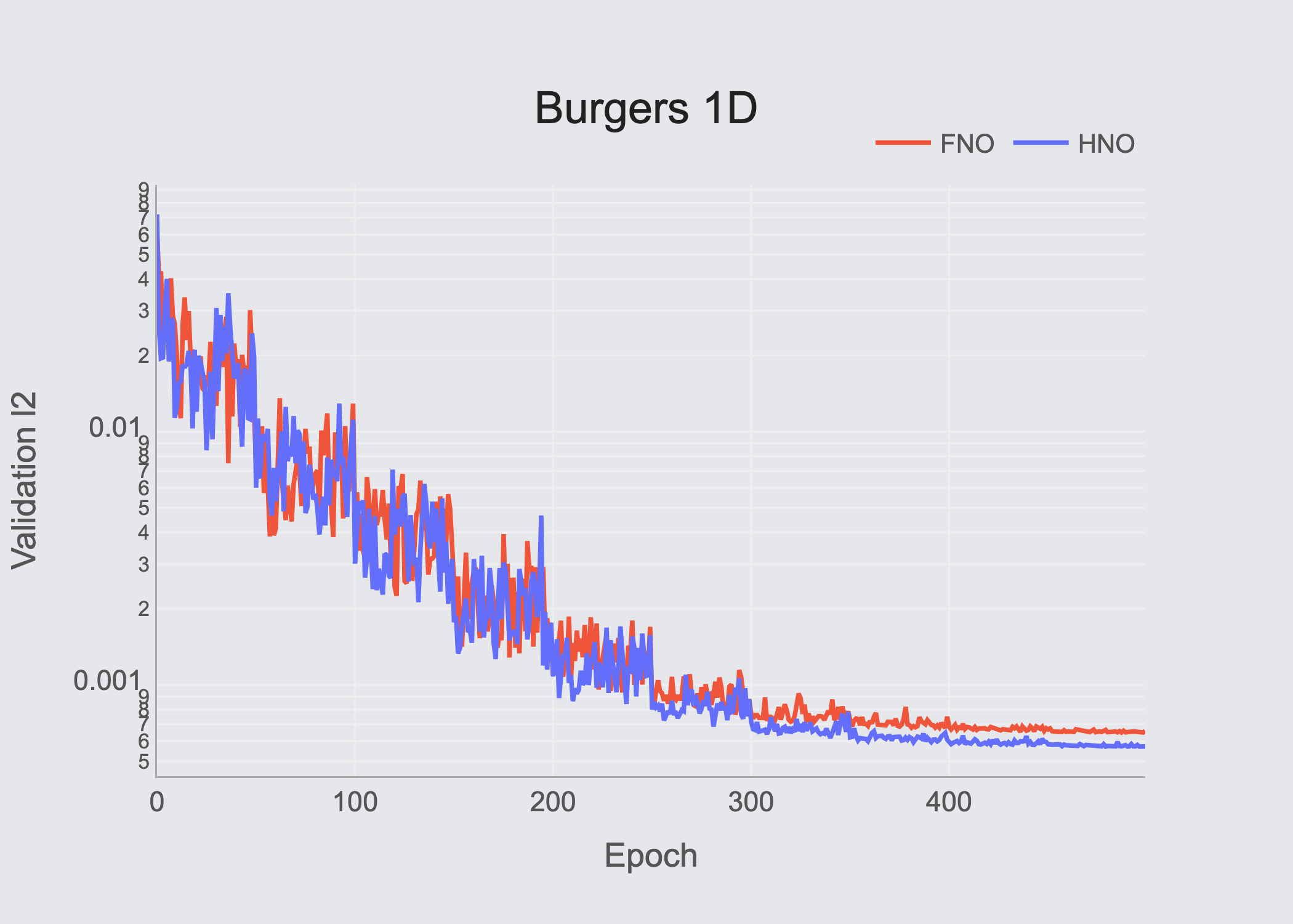
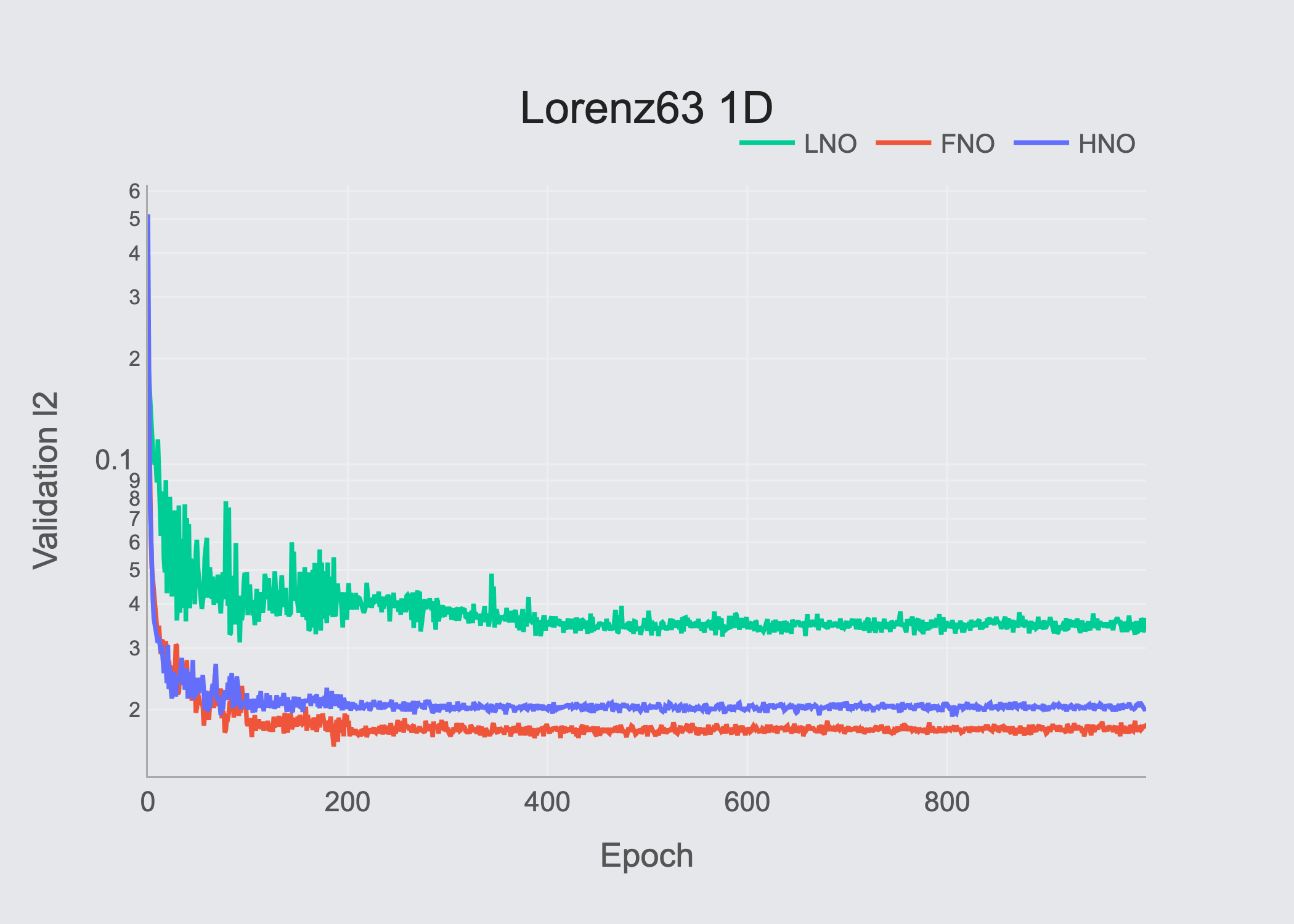
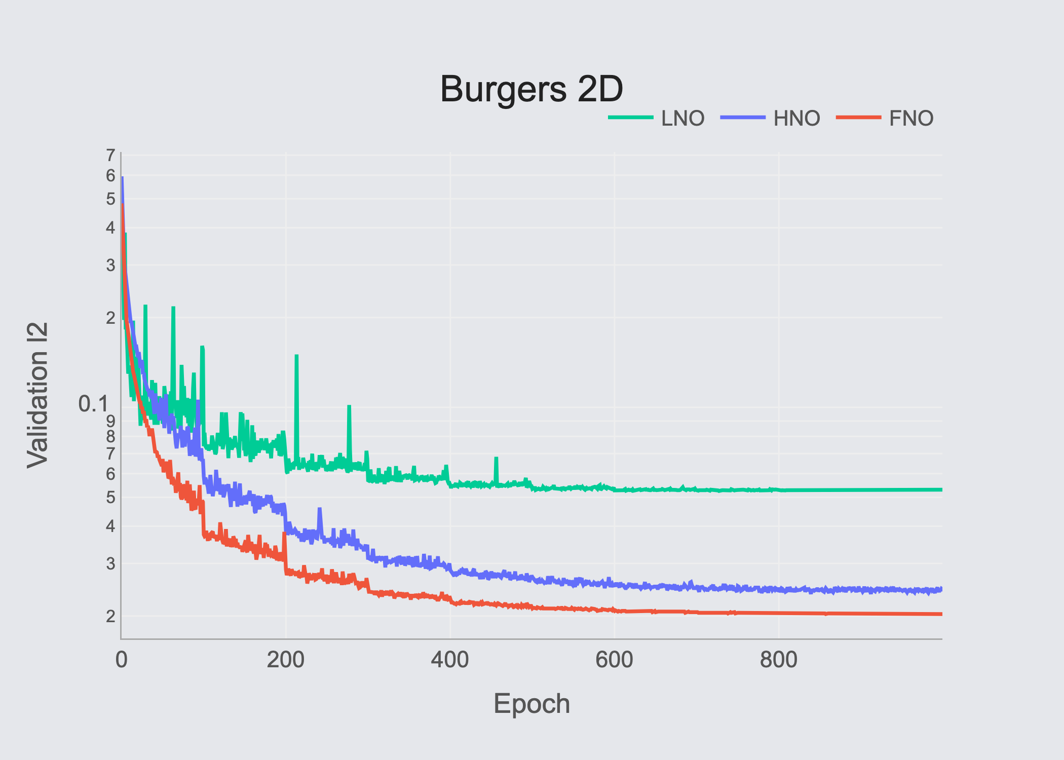
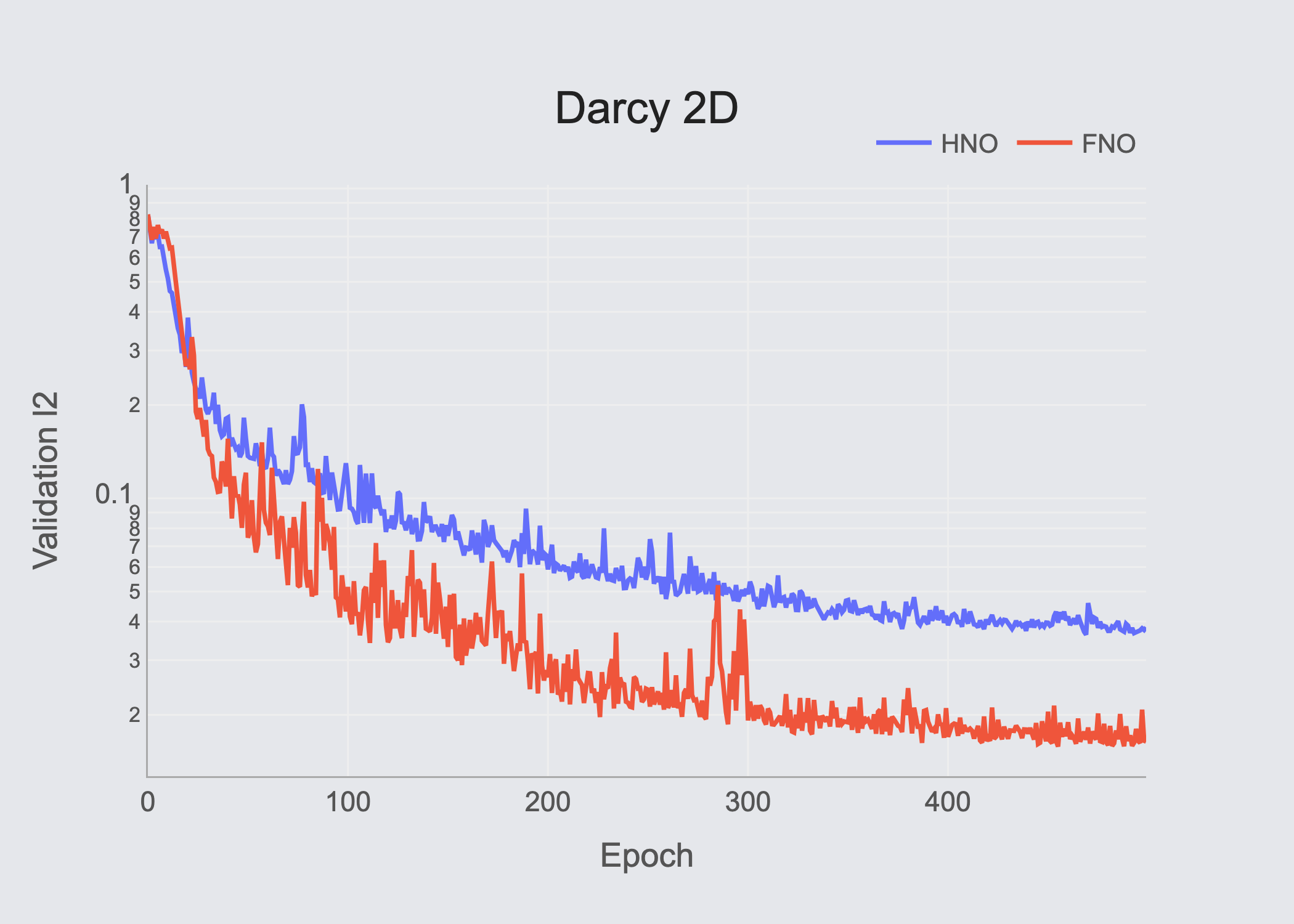
Table of results (Validation RMSE)

PDE	HNO	FNO	LNO
Burgers-1D	5.72×10⁻⁴	6.57×10⁻⁴	—
Lorenz63-1D	5.06×10⁻³	3.94×10⁻³	2.03×10⁻²
Burgers-2D	6.03×10⁻⁵	4.11×10⁻⁵	1.18×10⁻⁴
DarcyFlow-2D	3.83×10⁻²	1.64×10⁻²	—

Our experimental results show that all evaluated architectures show strong performance, while the proposed HNO & FNO perform stronger, with competitive differences.

This is where we see the strength of this method and motivates us to investigate further and research the more tailored use cases of the HNO in fields where other architectures struggle.

Ongoing Research

This article serves as an introduction to the Hilbert Neural Network concept. It presents some preliminary results to illustrate the mathematical background, architecture design, and performance through known benchmarks, sharing this information with the broader community.

Our next step is to expand the experimental scenarios and test the performance of HNO on other SciML applications, such as control and forecasting, where we’ve witnessed HNO outperforming other solutions.

We are also working on the mathematical aspects of the problem and trying to view the signal tensors in a different light, as well as testing new ideas such as channel eigen-decomposition to learn about other features of a signal that evolve in the time domain.

References

1. M. Raissi, P. Perdikaris, G. Karniadakis. “Physics informed deep learning (part i): Data-driven solutions of nonlinear partial differential equations,” in arXiv preprint arXiv:1711.10561, 2017.
2. L. Lu, P. Jin, G. Karniadakis. “Deeponet: Learning nonlinear operators for identifying differential equations based on the universal approximation theorem of operators,” in arXiv preprint arXiv:1910.03193, 2019.
3. Kovachki, N., et al. “Neural operator: Learning maps between function spaces with applications to pdes,” in Journal of Machine Learning Research, vol. 24, no. 89, pp. 1–97, 2023.
4. Li, Z., et al. “Fourier neural operator for parametric partial differential equations,” in arXiv preprint arXiv:2010.08895, 2020.
5. Q. Cao, S. Goswami, G. Karniadakis. “Laplace neural operator for solving differential equations,” in Nature Machine Intelligence, vol. 6, no. 6, pp. 631–640, 2024.

Acknowledgement

AI tools were used in the text editing of this article to rephrase some paragraph, grammer strength, and having more clear sentence structure.